In some cases, the orthomosaic product from processing Micasense data in Metashape comes out as dark. This article details a way to extract a false-color image with adjusted brightness for visualization and quality control.
The workflow described here is applicable for both Red Edge and Altum datasets processed using Agisoft Metashape Pro. The final output is a false-color image with each band scaled to capture the features of the scene more explicitly. Note that the product is not viable for radiometric applications. It is only meant to be used for visualization purposes, either for instructive scene maps or for quality control.
Part 1. Why is this Workflow Needed?
When processing in Metashape with images calibrated using both the reflectance panel and the downwelling light sensor of the payload, the final orthomosaic output can be quite dark. The band values themselves are radiometrically valid and are useful for the generation of relevant indices but not so much for visual inspection. The image below shows an example of such an orthomosiac.
 Multiple factors can result in a dark orthomosaic. One is the presence of highly reflective objects in the scene. This skews the scaling of the reflectance values due to the oversaturation of certain pixels.
The workflow that is described in the subsequent parts assumes that you have already processed the images from calibration to ortho generation following the recommended workflow in the Knowledge Base. As such, only the extra steps for the false-color image creation will be described. In this example, the intended false-color image is RGB. You can also do this for NIR-G-B, or whatever 3-band combination you need for visualization.
Part 2. Generating a Brighter False-Color Image
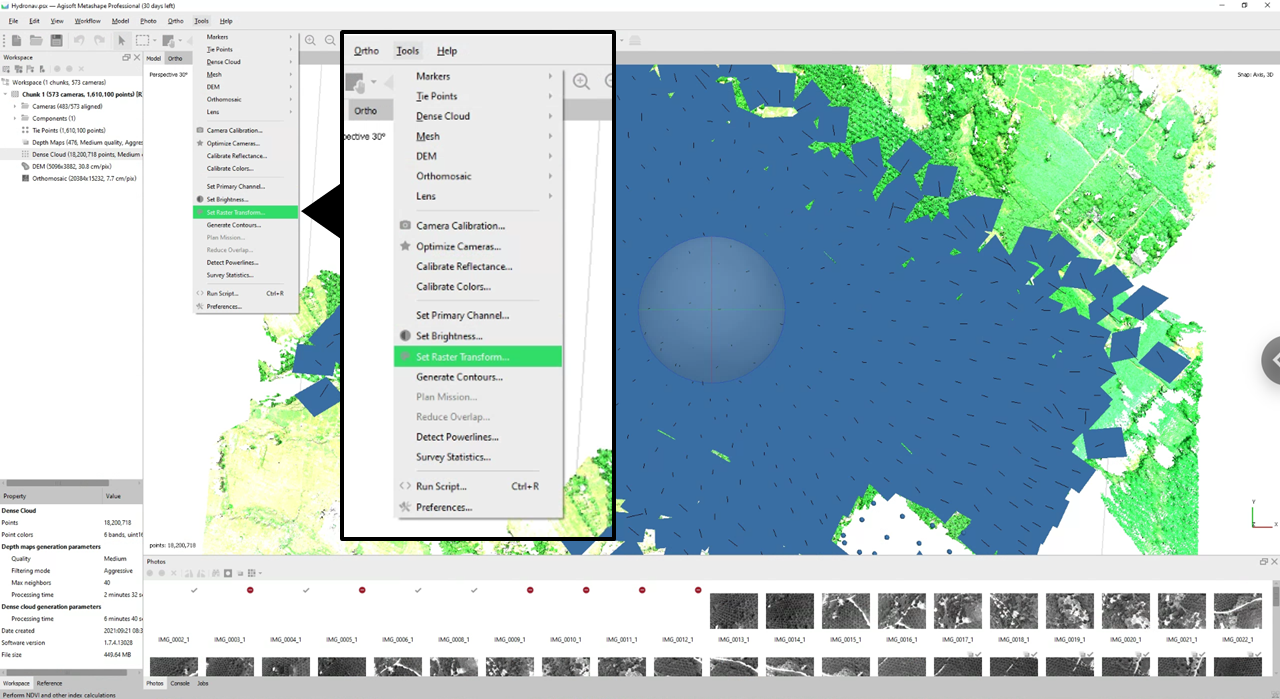
Once you have your 5- or 6-band orthomosaic produced and saved, you can now follow this process. Start by going to Tools > Raster Transformation.
In the prompt that opens, you want to order the bands accordingly (e.g. Red, Green, Blue) and then use a scaling factor to improve the brightness. The reflectance values stored in the bands are 16-bit integers. This means that they run from 0 to 65,535. However, by design, 100% reflectance will only correspond to the median of the range, which is 32,768. In our case, we want to both normalize and scale the values to adjust for brightness. The scaling factor we are going to use is 0.6 as this has been shown to produce an orthomosaic that crisply captures the scene features. The transformation is shown below.
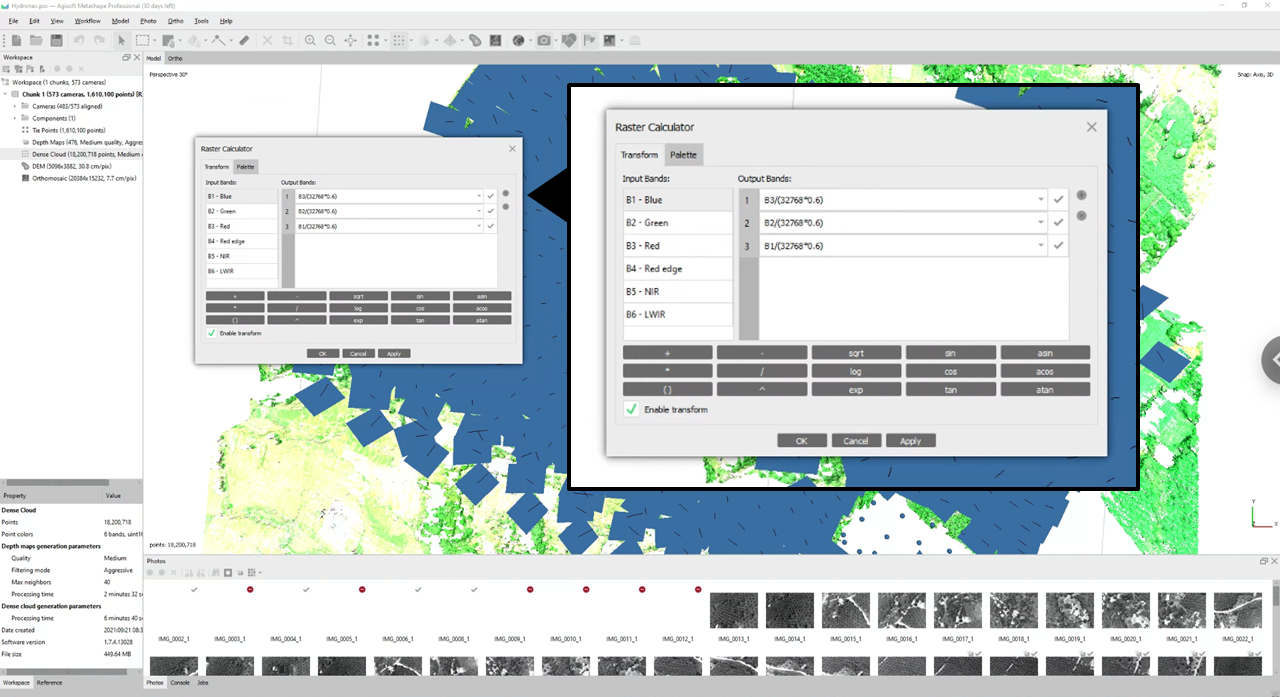
The band transformations are as follows:
B1 = B3/(32786*0.6)
B2 = B2/(32786*0.6)
B3 = B1/(32786*0.6)
Note: For a False-Color other than RGB, the band sequence will be different. As an example, for a NIR-G-B image, you will want:
B1 = B5/(32786*0.6)
B2 = B2/(32786*0.6)
B3 = B1/(32786*0.6)
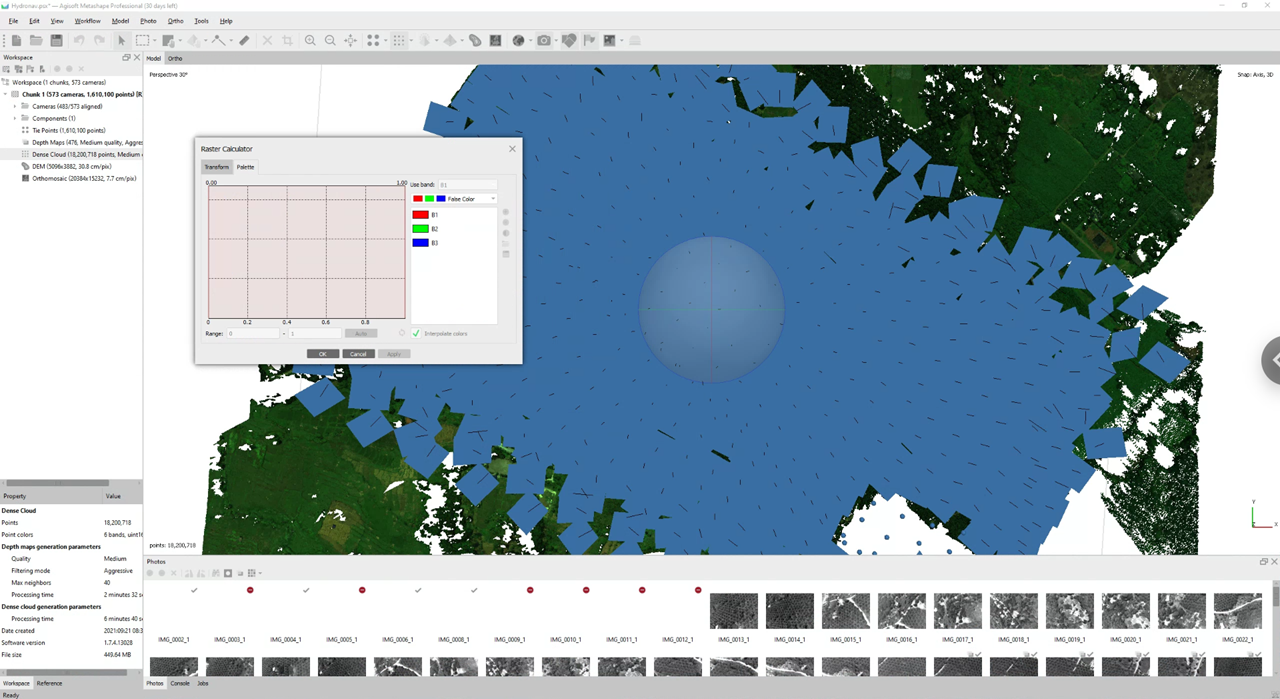
After setting up the transformation, click Apply and go to Palette. To see what the resulting orthomosaic will look like, change the display setting from Heat to False Color then click OK.
If you double-click on the Orthomosaic under the Components section on the left pane, it will direct you to the Ortho tab and this will display the resulting false-color product that you can now export.
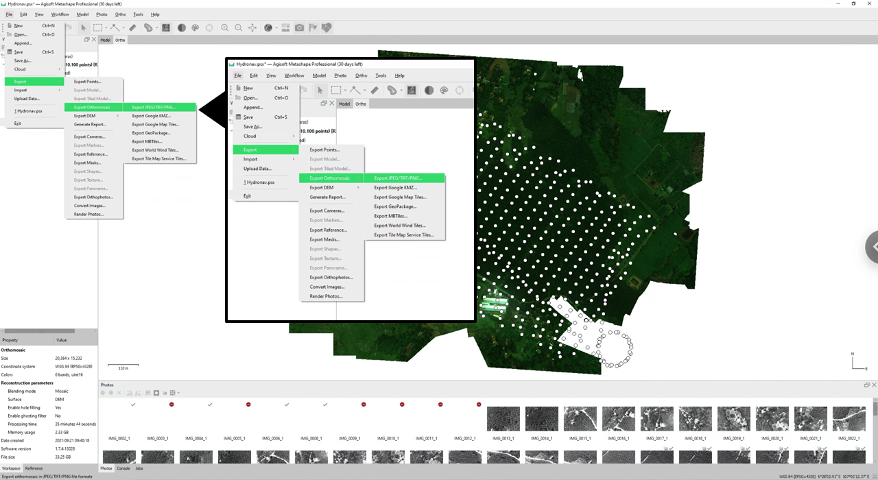
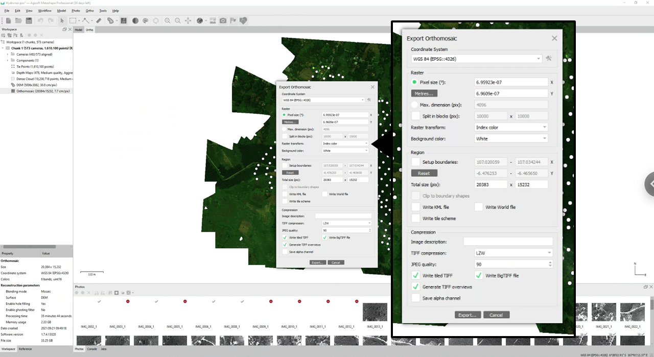
To export the resulting product, go to File > Export Orthomosaic > Export JPEG/TIFF/PNG. On the dialog box that pops up, make sure to select Index Color under Raster Transform. This will create the False Color product that you need. If you kept it at None, you’ll just get the typical 5- or 6-band product.
Part 3. Evaluating the Final Output
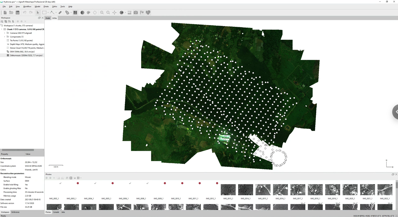
As a final step, to confirm that you have what you need, use your software of choice to view the resulting orthomosaic. It should now be brighter and more defined than the original product, as shown in the image below.
 Notice the highly reflective feature near the bottom of the image. This likely contributed to why the output orthomosaic was dark.